


Introduction: Why Traditional Algorithms Are Not Always Enough
When students first learn algorithms, they are usually introduced to clear, step-by-step procedures that promise a correct answer every time. These approaches work well for small and well-defined problems. However, during classroom discussions, it has become clear that many real-world complex problems do not fit neatly into this structure.
Some problems have extremely large solution spaces with respect to time and space complexity. Others involve uncertainty, incomplete information, or conflicting objectives. In such cases, traditional algorithms may either take too long or fail to produce practical results. This is where the idea of evolutionary algorithms becomes important, as they help identify an optimum solution from multiple available options.
While teaching optimization and artificial intelligence concepts, I often emphasize that evolutionary algorithms do not aim for perfection. Instead, they aim for improvement in the overall performance of a system by accomplishing the optimum expected result. This shift in thinking is crucial for students transitioning from theoretical problem-solving to real-world system design.
Problems in Hill Climbing Algorithm
Local Maximum
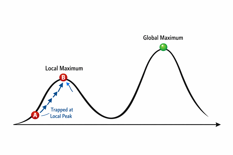
- Hill Climbing Algorithm is a local search algorithm.
- Greedy Approach
- No backtracking
In the Hill Climbing algorithm, the following steps are used to determine the best possible solution:
- Evaluate the initial state
- In this case, Beta = 1, where Beta is the beam width.
- Loop until a solution is found or there are no operators left.
- Select and apply a new operator
- Evaluate the new state. If it is the goal state, then quit.
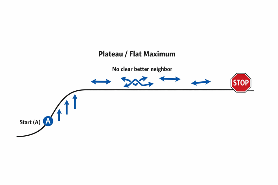
Plateau / Flat Maximum

Simulated Annealing vs Hill Climbing
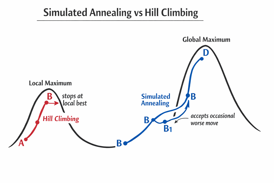
Simulated Annealing allows downward steps, unlike Hill Climbing. In the figure above, Hill Climbing moves upward from point A to point B. Once it reaches B, which is a local maximum, it stops because it assumes that the highest nearby point has been reached. However, the best solution in the figure is at point D, which represents the global maximum.
To overcome this limitation, Simulated Annealing does not stop at point B. It may move from B to B1, accepting a temporary downward step, and then continue toward point D, the global maximum. This gives the algorithm a better chance of finding the best possible outcome.
While Hill Climbing works well for simple or well-structured problems, its limitations become clear as complexity increases. The algorithm can easily become trapped in a local optimum. Once it reaches a point where all nearby moves appear worse, the search stops, even though a better solution may exist elsewhere.
Simulated Annealing addresses this limitation by allowing occasional acceptance of worse solutions. At first, this idea feels counterintuitive to learners. However, when related to real-life decision-making, it becomes easier to grasp. People often accept short-term discomfort or setbacks to achieve better long-term outcomes. Simulated Annealing follows the same reasoning.
The algorithm introduces controlled randomness through the concept of temperature. In the early stages, higher temperature allows exploration of the search space, even if some moves reduce solution quality. Over time, the temperature is gradually reduced, making the algorithm more selective and stable.
| Simulated Annealing | Hill Climbing |
| Maintains an annealing schedule using temperature. | Does not use an annealing schedule. |
| Can accept worse moves temporarily to escape local optima. | Accepts only better moves and may stop at a local optimum. |
| Maintains the best state found during the search. | Moves greedily toward the best immediate neighbor. |
As temperature decreases, Simulated Annealing slowly begins to behave like Hill Climbing. This transition helps balance exploration and exploitation in a structured way. Instead of blindly improving or randomly exploring, the algorithm learns when to experiment and when to settle.
From an academic perspective, Simulated Annealing is useful for explaining important ideas such as local versus global optima, the role of randomness in intelligent systems, and the trade-off between accuracy and efficiency. These ideas align well with Artificial Intelligence and algorithm analysis topics studied in both BCA and MCA programs.
Simulated Annealing also encourages a broader view of intelligence. It teaches that intelligent behavior does not always mean choosing the best immediate option. Sometimes, flexibility and patience lead to better results. This insight is valuable not only in algorithm design but also in understanding real-world problem-solving.
Advantages
- Easy to code for complex problems
- Gives good solutions
- Statistically guarantees finding optimal solution
Disadvantages
- It is a slow process
- Can’t say whether an optimal solution is found
- In order to determine the optimal solution some other methods are required
Discussion Questions
- Why does Hill Climbing fail in certain optimization problems, and how does Simulated Annealing overcome this limitation?
- How does the concept of temperature influence decision-making in Simulated Annealing?
- In what types of problems would Simulated Annealing be preferred over Hill Climbing?
- How does controlled randomness contribute to intelligent problem solving?
Course Relevance
Simulated Annealing connects strongly with topics taught in Artificial Intelligence, Design and Analysis of Algorithms, and Optimization Techniques. For BCA students, it builds conceptual understanding of search strategies and algorithm behavior. For MCA students, it supports advanced discussions on optimization, heuristic search, and real-world problem modeling.
Teaching Notes
- Introduce Hill Climbing first to establish baseline understanding.
- Use real-life examples to explain why accepting worse solutions can be beneficial.
- Focus on conceptual flow rather than mathematical formulation in early stages.